Local and global theorems
34) Local and global theorems.
Theorem. For any point  T there exists a fundamental matrix solution
  defined in some small neighborhood U of
 ![]() .
.
Proof. The linear vector-function (t, x) ![]()
![]() is holomorphic everywhere on T ×
is holomorphic everywhere on T × ![]() . By the local existence theorem, for any initial condition (
. By the local existence theorem, for any initial condition (![]() ,
,![]() )
) ![]() T ×
T × ![]() there exists a holomorphic vector solution
there exists a holomorphic vector solution  defined on some neighborhood of
 ![]() , meeting the condition
, meeting the condition  . Choose n solutions satisfying n linear independent initial conditions at
 ![]() , arranged as columns of a square matrix and considered on their common domain.
, arranged as columns of a square matrix and considered on their common domain.
By construction,  , hence the holomorphic matrix is holomorphically invertible in some neighborhood
 ![]() of the point
of the point ![]() .
. ![]()
Theorem. (global existence theorem). A linear system on a Riemann surface T admits a fundamental solution in any simply connected subdomain 
Proof. Choose a base point  and let
  be a local fundamental matrix solution at this point. We extend it to an arbitrary point
  .
.
Since ![]() is connected, there exists a compact piecewise smooth curve (path) γ connecting
is connected, there exists a compact piecewise smooth curve (path) γ connecting ![]() with
with ![]() . γ can be covered by
. γ can be covered by  carrying the respective local fundamental matrix solutions
 , such that
  are connected, and
  if and only if |i − j|
 ![]() 1.
1.
Assume that  satisfy
  ,
, ![]() ,
,  . Then
  ,
, ![]()
Agree on the intersections:
 ,
, 
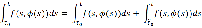
the solution can be explicitly constructed:

![]() .
.
This completes the proof of existence of analytic continuation of solutions along paths. ![]()
35) Analyticity and differentiation of solutions.
If f ‘(x0) exists, then for x close to x0, we have
![]()
This is the "linear approximation" done via the tangent line. Obviously this implies
 ,
,
which means that  is continuous at
![]() . Thus there is a link between continuity and differentiability: If a function is differentiable at a point, it is also continuous there. Consequently, there is no need to investigate for differentiability at a point, if the function fails to be continuous at that point.
. Thus there is a link between continuity and differentiability: If a function is differentiable at a point, it is also continuous there. Consequently, there is no need to investigate for differentiability at a point, if the function fails to be continuous at that point.
Note that a function may be continuous but not differentiable, the absolute value function at  is the archetypical example.
This relationship between differentiability and continuity is local. But a global property also holds. Indeed, let ![]() be a differentiable function on an interval
be a differentiable function on an interval ![]() . Assume that
. Assume that ![]() is bounded on
is bounded on ![]() , that is there exists
, that is there exists  such that
 for any
 ![]()
The Mean Value Theorem will then imply that
![]()
for any  . This is the definition of Lipschitz continuity. In other words, if
 ![]() is bounded then
is bounded then  is a Lipschitzian function. Conversely, it is also true that Lipschitzian functions have bounded first derivatives, when they exist. Since Lipschitzian functions are uniformly continuous, then is uniformly continuous provided
  is bounded.
Nevertheless, a function may be uniformly continuous without having a bounded derivative. For example,  is uniformly continuous on [0,1], but its derivative is not bounded on [0,1], since the function has a vertical tangent at 0.
36) Solution continuity of parameters and initial data.
Theorem. Suppose that ƒ and ![]() are continuous and bounded in a given region U. Let
are continuous and bounded in a given region U. Let  be a solution of (1) passing through
 ![]() ,
, ![]() and
and  be a solution of (1) passing through (
 . Suppose that ϕ and ψ exist on some integral I.
Then, for each ε > 0, there exists δ > 0 such that if |t — ![]() | < δ and ||
| < δ and || || < δ, then
||ϕ(t) – ψ(![]() )|| < ε, for t,
)|| < ε, for t, ![]() ∈ I.
∈ I.
Proof. Since ϕ is the solution of (1) through the point ( ), we have, for all t ∈ I,
ϕ(t)= ![]() +
+  (2)
(2)
As ψ is the solution of (1) through the point (![]() ,
,![]() ), we have, for all t ∈ I,
), we have, for all t ∈ I,
ψ(t)= ![]() +
+  (3)
(3)
Since
subtracting (3) from (2) gives
|| ϕ(t) – ψ(t) || ![]() ||
|| || + ||
 ||+||
||+|| ||
||
Using the boundedness assumptions on ƒ and ![]() to evaluate the right hand side of the latter inequation, we obtain
to evaluate the right hand side of the latter inequation, we obtain
|| ϕ(t) – ψ(t) || ![]() |||| +M |
|||| +M | | + K
| + K
If || < δ, || || <δ, then we have
|| ϕ(t) – ψ(t) || ![]() +Mδ + K ||
+Mδ + K || 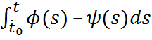 || (4)
Applying Gronwall’s inequality to (4) gives
||ϕ(t) – ψ(![]() )||
)||![]() ||ϕ(t) – ψ(t)||
||ϕ(t) – ψ(t)||![]() ||ψ(t) – ψ(
||ψ(t) – ψ( ![]() )||
)|| 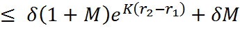
Now, given ε > 0, we need only choose  ε/[M + (1+
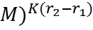 ] to obtain the desired inequality, completing the proof.
37. Fundamental system of solutions
Definition. System of n linearly independent solutions ![]() (t),
(t), ![]() (t), …,
(t), …, ![]() (t)
(t)
of system 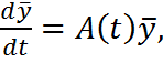 is called a fundamental system of solutions or basis.
Theorem. The system  has a fundamental system of solutions. If
![]() (t),
(t), ![]() (t), …,
(t), …, ![]() (t) is basis, then the general solution has the form
(t) is basis, then the general solution has the form
 where
where  are arbitrary constants.
Concept of the fundamental matrix. Ostrogradsky-Liouville formula.
We consider the system
![]()
of n arbitrary vector solutions of the vector equation  and form a matrix of the order nxn
Y(t) =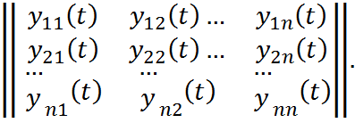
and the Wronskian. If the system of vectors 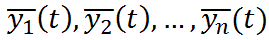 is linearly independent, then detY(t)=W(t)does not vanish for any value t of the interval of continuity of the matrix A(t). In this case the matrix Y(t) is called an integral or a fundamental matrix for the system
 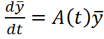 . If Y(
![]() )= E, where E is the unit matrix, the matrix is called integral normalized at the point t=
)= E, where E is the unit matrix, the matrix is called integral normalized at the point t=![]() .
.